I recently wanted to create some randomized data for use in a simple proof-of-concept experiment.  I was creating a simulated population of users in various locations around the world, and so I needed to take a few hundred rows and randomly assign them one of a dozen different regions.

The trick was that to make the data realistic, I didn’t want to a truly random distribution. I wanted a “headquarters” that would have a very large population of users, a few regional locations that would have smaller but still significant numbers, and then a bunch of “satellite” locations that would have just a handful.

If you just use a combination of the “CHOOSE” and “RANDBETWEEN” functions in Excel, you get an even distribution across all the options.  This would make my data look funny – rows tagged for my made-up headquarters in “New York City” would have roughly the same number of rows as the ones tagged with my made-up satellite office in “Quito, Ecuador”.  How could I get a more realistic distribution but still have it be randomly generated?

I found a solution by using VLOOKUP to specify ranges for each location, with larger ranges for locations that should have more rows, and then using RANDBETWEEN to drive the lookups.

First, I set up a distribution.  I chose a range of 0-99, and then allocated chunks of it to various locations as follows:

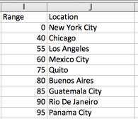
The data in the left column specifies the range

The way to read this is that 40% of the data will be in my headquarters in New York City (i.e. 0-39). My regional locations of Chicago and Mexico City will each get 15% (hence sequential values of 55, and 75), and then my satellite offices of Los Angeles, Quito, Buenos Aires, Guatemala City, Rio de Janeiro, and Panama City will each get 5%.  The only confusing thing about it is that each row has its starting number, not its ending number, so to get a sense of the size of a range, you need to compare the values of the each row and the one after it.

Now, I can use the VLOOKUP function to specify lookups into that table.  Using the optional “range lookup” option, I can specify that excel should choose the row that falls into the range if there is no exact match.

The notation is “=VLOOKUP(30,$I$2:$J$10, 2, 1)”.  The options are as follows:

• The first option (30) specifies that the value “30” should be looked up.  I’ve hardcoded the value, but this can reference another cell
• The second option ($I$2:$J$10) represents the array of cells that hold my location mappings.  Column I has the ranges, and column J has the values
• The third option (2) specifies the output column.  So, I am looking up values in column 1 (I), but I want it to return the value in column 2 (J)
• The fourth option (1) instructs excel to use range lookups.  In this example, there is no row with a “30” in it, so Excel should assume these are ranges and use the closest smaller match, which will be the row 0

So, if I put the value “30” into the first argument, it will give me “New York City”, but if I put “41”, it will give me “Chicago”.

I can now pair this up with a whole bunch of RANDBETWEEN(0,99) values and generate a sample set that follows my specified distribution, giving more rows with the headquarters of New York City, some rows to the regional locations, and just a few rows to the satellite offices:

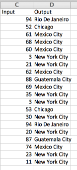
Using VLOOKUP, I can use the RANDBETWEEN generated values in Column C to fill in the correct matching locations in column D

I’ve shown just 20 examples above, so as with any small random distribution there are fluctuations (a little more Mexico City than I would expect and no Los Angeles), but if you generate a few hundred the distribution will become closer and closer to the ranges I have specified.

Okay, so far, so good.  But now I want to take it a step further.

What if I want a second column that will specify region (North American, Central America, or South America)?  The data is all random, so I could create a second randomized column for the region.  However, if I just replicate what I did above, the data won’t make sense.  Since each random value is generated independently, I will get non-sensical combinations like a location of “New York City” but a region of “Central America”.

The solution is to have a second VLOOKUP based on the original randomized location value to choose an appropriate region.

So, I start by adding a column to the distribution data to associate a region with each location:

To avoid mismatches, I add a region for each location

Then, I add a new VLOOKUP column to my dataset, where the new column is a VLOOKUP of the randomly generated value into the location/region list. This time, I turn the “range lookup” option to 0, since I don’t expect the data to be sorted and I will always have an exact match [VLOOKUP(D2,$J$1:$K$10,2,0)]:

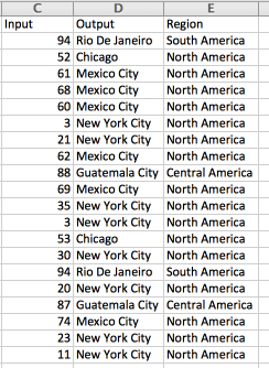
VLOOKUPs are chained. The Output column was randomly generated, and the Region column does a VLOOKUP with whatever value was chosen.

Now, my randomized data makes sense; the selection of locations follows a meaningful distribution, and the “dependent” columns are properly selected rather than just being separate random decisions.

None of this is rocket science, obviously, and I am sure there are a hundred other ways to do this as well using some of the more advanced tools hidden inside Excel. However, this way is a quick and easy, so I figured I would document the recipe in case someone wants to follow it…

… and also so that I can refer back to it at some point down the road without having to recreate it from scratch.